Lecture 3

Bias, Variance and MSE 偏差、方差、均方差

• Consider a statistical model that is parameterized by \(\theta\) and that determines a probability distribution over observed data \(P(x \mid \theta)\)
• Consider a statistic \(\hat{\theta}\) that provides an estimate of \(\theta\) and is a function of observed data \(x \quad \hat{\theta}=f(x)\)
• E.g. for a Gaussian distribution with known variance, the average of a set of i.i.d data points is an estimate of the mean of the Gaussian
• Definition: the bias of an estimator \(\hat{\theta}\) is:

\[ \operatorname{Bias}_ \theta(\hat{\theta})=\mathbb{E}_{x \mid \theta}[\hat{\theta}]-\theta \]

• Definition: the variance of an estimator \(\hat{\theta}\) is:

\[ \operatorname{Var}(\hat{\theta})=\mathbb{E}_{x \mid \theta}\left[(\hat{\theta}-\mathbb{E}[\hat{\theta}])^2\right] \]

• Definition: mean squared error (MSE) of an estimator \(\hat{\theta}\) is:

\[ \operatorname{MSE}(\hat{\theta})=\operatorname{Var}(\hat{\theta})+\operatorname{Bias}_\theta(\hat{\theta})^2 \]

First-visit Monte Carlo

Initialize \(N(s)=0, G(s)=0 \forall s \in S\) Loop

• Sample episode \(i=s_{i, 1}, a_{i, 1}, r_{i, 1}, s_{i, 2}, a_{i, 2}, r_{i, 2}, \ldots, s_{i, T_i}\)
• Define \(G_{i, t}=r_{i, t}+\gamma r_{i, t+1}+\gamma^2 r_{i, t+2}+\cdots \gamma^{T_i-1} r_{i, T_i}\) as return from time step \(t\) onwards in ith episode
• For each state \(s\) visited in episode \(i\)
  • For first time \(t\) that state \(s\) is visited in episode \(i\)
    • Increment counter of total first visits: \(N(s)=N(s)+1\)
    • Increment total return \(G(s)=G(s)+G_{i, t}\)
    • Update estimate \(V^\pi(s)=G(s) / N(s)\)

Properties:

• \(V^\pi\) estimator is an unbiased estimator of true \(\mathbb{E}_\pi\left[G_t \mid s_t=s\right]\)
• By law of large numbers, as \(N(s) \rightarrow \infty, V^\pi(s) \rightarrow \mathbb{E}_\pi\left[G_t \mid s_t=s\right]\)

first vist monte carlo指的是第一次见到状态s时的时刻开始的累积reward，比如一共10个时刻，看到状态s时是第三个时刻，那么该episode只算3-7步的累积回报。

FVMC是无偏估计因为其得到的估计值就是每一个episode中遇见状态s的实际回报值的均值估计，因此增加无限个episode就会使估计值等于实际值。

Every-visit Monte Carlo

Initialize \(N(s)=0, G(s)=0 \forall s \in S\) Loop

• Sample episode \(i=s_{i, 1}, a_{i, 1}, r_{i, 1}, s_{i, 2}, a_{i, 2}, r_{i, 2}, \ldots, s_{i, T_i}\)
• Define \(G_{i, t}=r_{i, t}+\gamma r_{i, t+1}+\gamma^2 r_{i, t+2}+\cdots \gamma^{T_i-1} r_{i, T_i}\) as return from time step \(t\) onwards in ith episode
• For each state \(s\) visited in episode \(i\)
  • For every time \(t\) that state \(s\) is visited in episode \(i\)
    • Increment counter of total first visits: \(N(s)=N(s)+1\)
    • Increment total return \(G(s)=G(s)+G_{i, t}\)
    • Update estimate \(V^\pi(s)=G(s) / N(s)\)

Properties:

• \(V^\pi\) estimator is an biased estimator of true \(\mathbb{E}_\pi\left[G_t \mid s_t=s\right]\)
• but consistent estimator and often has better MSE

Every-visit Monte Carlo是将每一次遇到状态s后累积的reward都累加，除以遇见状态s的次数得到estimated return，相当于在一个episode中重复使用first-visit monte carlo，求平均return，因此是有偏差的估计，因为其得到的估计值并不是实际的观测值，而是一个基于多次在一个episode中观测多次某一个状态s的平均值（虽然\(N(s)\)加到了总的计数counter上，但是结果是一样的，相当于在一个episode中平均了对一个状态的return）。

蒙特卡洛递增策略评估

Incremental Monte Carlo (MC) On Policy Evaluation ： After each episode \(i=s_{i, 1}, a_{i, 1}, r_{i, 1}, s_{i, 2}, a_{i, 2}, r_{i, 2}, \ldots\)

• Define \(G_{i, t}=r_{i, t}+\gamma r_{i, t+1}+\gamma^2 r_{i, t+2}+\cdots\) as return from time step \(t\) onwards in ith episode
• For state \(s\) visited at time step \(t\) in episode \(i\)
• Increment counter of total first visits: \(N(s)=N(s)+1\)
• Update estimate

\[ \begin{equation} \begin{aligned} V^\pi(s) &=V^\pi(s) \frac{N(s)-1}{N(s)}+\frac{G_{i, t}}{N(s)}\\ &=V^\pi(s)+\frac{1}{N(s)}\left(G_{i, t}-V^\pi(s)\right)\\ &=\alpha \left(G_{i, t}-V^\pi(s)\right) \end{aligned} \end{equation} \]

其中\(\frac{1}{N(s)}\)可以当成学习速率\(\alpha\)

算法：

Initialize \(N(s)=0, G(s)=0 \forall s \in S\) Loop

• Sample episode \(i=s_{i, 1}, a_{i, 1}, r_{i, 1}, s_{i, 2}, a_{i, 2}, r_{i, 2}, \ldots, s_{i, T_i}\)
• Define \(G_{i, t}=r_{i, t}+\gamma r_{i, t+1}+\gamma^2 r_{i, t+2}+\cdots \gamma^{T_i-1} r_{i, T_i}\) as return from time step \(t\) onwards in \(i\) th episode
• For state \(s\) visited at time step \(t\) in episode \(i\)
• Increment counter of total first visits: \(N(s)=N(s)+1\)
• Update estimate

\[ V^\pi(s)=V^\pi(s)+\alpha\left(G_{i, t}-V^\pi(s)\right) \]

• \(\alpha=\frac{1}{N(s)}\) : identical to every visit MC
• \(\alpha>\frac{1}{N(s)}\) : forget older data, helpful for non-stationary domains

一个例子：

• 火星车的状态的奖励值s1-s7为: \(\mathrm{R}=\left[\begin{array}{llllll}1 & 0 & 0 & 0 & 0 & 0\end{array}+10\right]\) for any action
• \(\pi(s)=a_1 \quad \forall s, \quad \gamma \equiv 1\). any action from \(s_1\) and \(s_7\) terminates episode
• 轨迹为 \(=\left(s_3, a_1, 0, s_2, a_1, 0, s_2, a_1, 0, s_1, a_1, 1\right.\), terminal \()\)

1. 求First visit MC 算法下的所有状态s 的状态估计值\(V\) ?

   对于First Visit MC 有\(V = [1, 1, 1, 0, 0, 0, 0]\) ,因为除了$s_1,s_2,s_3 \(意外其他状态没有采样，在轨迹中\)s_1$在最后，因此所有采样的状态的First visit return都是1（所有在轨迹中的状态只遇见过一次）

2. 求\(s_2\)的 ever-visit MC的状态估计值

   \(V(s_2) = 1\) ，因为即便在轨迹中\(s_2\)出现两次，但是由于\(\gamma=1\)，terminal reward也是1，所以状态值为\(\frac{1+1}{2}=1\)

对状态\(s\)更新，就是利用当前对状态\(s\)的估计值，加上从\(s\)之后到T步的所有reward的return \(G_{i,t} = r_{i, t}+\gamma r_{i, t+1}+\gamma^2 r_{i, t+2}+\cdots \gamma^{T_i-1} r_{i, T_i}\) ,与当前的估计值的差值并乘以一个学习率\(\alpha(G_{i,t}-V^{\pi}(s))\)得到。

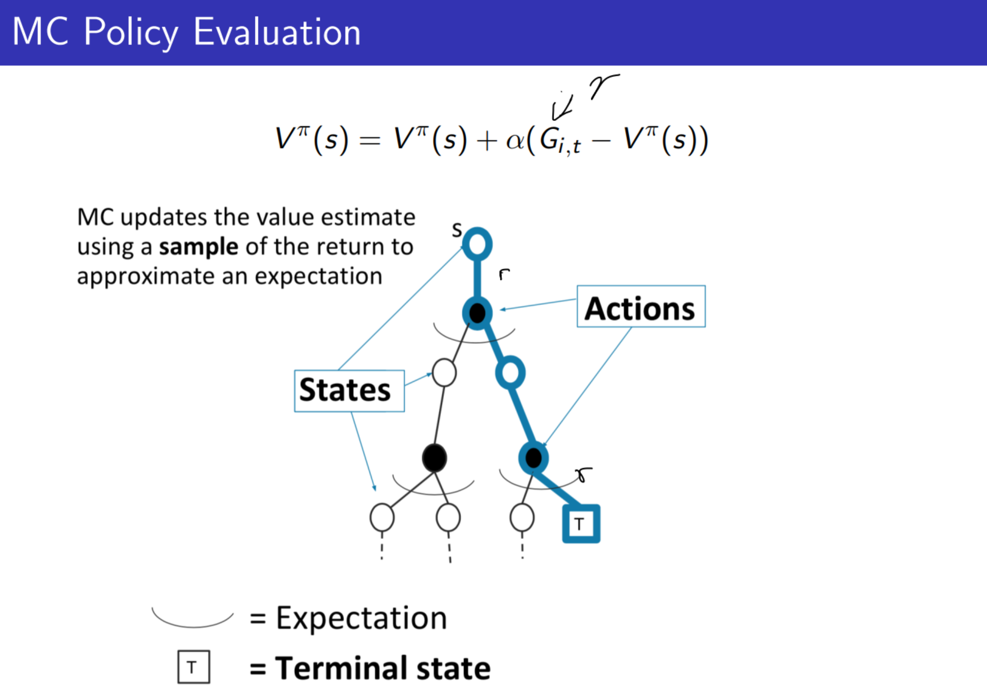
MC 方法总结而言，就是认为状态值的更新有赖于未来的奖励和当前对状态估计的差值，这种方法的缺点是需要将一个episode整个给过完（称为采样），得到每一个的奖励，使用First visit 或者Every visit 的方法得到return \(G\) 然后利用return和当前对起始状态值的估计的差值进行学习。MC方法不一定能够学习到每一个状态值，因为采样轨迹可能不包含某些状态，比如在围棋的状态树中，进行一次轨迹采样仅仅代表一条支路，但是整个围棋状态空间中包含的潜在可采样的轨迹是几何级别的，因此不可能将所有的轨迹（可能性）都进行一遍。

缺点：

1. 有较高的偏差
2. 需要完整的episode来更新value function

TD Policy evaluation TD(0)

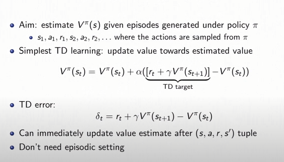
TD learning的思想很简单，相比于MC方法，TD方法不需要进行完整个episode才对状态值进行更新，而是每进行一步就可以对当前状态值进行更新。TDlearning之所以被称之为 bootstraping，是因为公式里的TD error部分使用当前步的策略来估计下一个状态的状态值，即\(V^{\pi}(s_{t+1})\)部分是使用的当前策略\(\pi\)估计下一个时刻\(s_{t+1}\)的策略值，为什么这样叫做bootstrap呢？因为每一个时刻的策略实际上是跟当前时刻的状态值绑定的，就是说如果状态值改变，那么选择动作的策略也会有响应的变化（也可能结果不变）,在每一步中这种变化可能会很小，但是依然是与当前时刻的状态值绑定的，用下一时刻状态所对应到当前时刻策略下的状态值当做下一时刻的该状态的状态值，就理所当然是自己更新了自己，即“自举”。

TD(0):最简单形式的TD learning

\[ V^\pi\left(s_t\right)=V^\pi\left(s_t\right)+\alpha\left(\left[r_t+\gamma V^\pi\left(s_{t+1}\right)\right]-V^\pi\left(s_t\right)\right) \]

TD error:

\[ \delta_t=r_t+\gamma V^\pi\left(s_{t+1}\right)-V^\pi\left(s_t\right) \]

接上面火星车的例子，同样的配置，如果换成是TD 方法则过程如下：

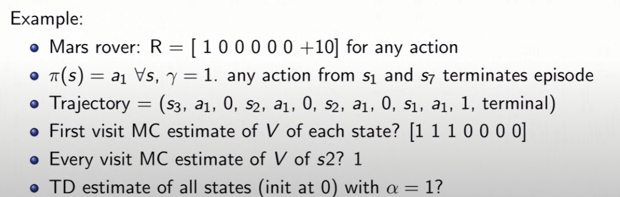
除了状态\(s_1\)以外，其余的状态均没有被更新

\[ \begin{array}{lllll} V\left(s_3\right)=0 & s_3 & a_1 & 0 & s_2 \\ V\left(s_2\right)=0 & s_2 & a_1 & 0 & s_2 \\ V\left(s_2\right)=0 & s_2 & a_1 & 0 & s_1 \\ V\left(s_1\right)=1 & s_1 & a_1 & +1 & \text { terminal } \end{array} \]

结果则是从\(s_1 \to s_7\) 状态值更新为：\([1,0,0,0,0,0,0]\)

• TD 是biased(有偏估计)!

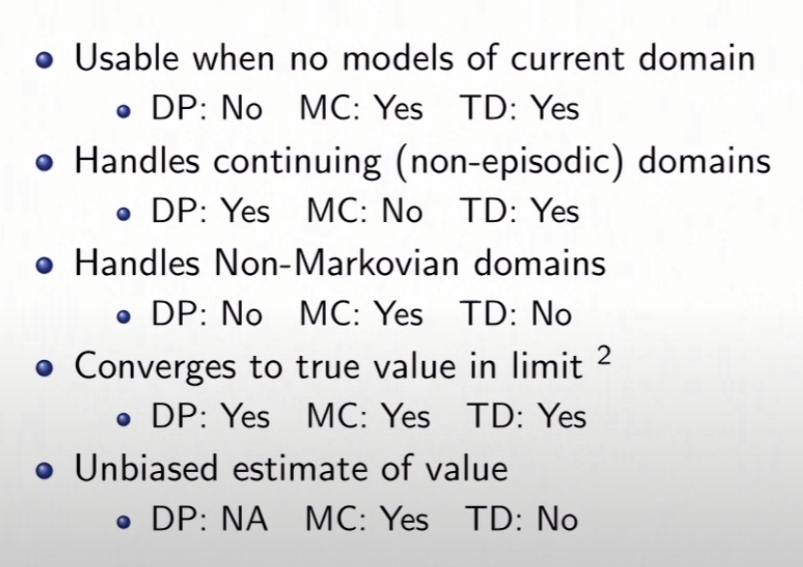
• 三种基础方法的总结