Flocking for Multi-Agent Dynamic Systems: Algorithms and Theory

In 1986, Reynolds introduced three heuristic rules that led to creation of the first computer animation of flocking [5]. Here, are the three flocking rules of Reynolds

1. Flock Centering: attempt to stay close to nearby flock mates; 和邻居接近
2. Collision Avoidance: avoid collisions with nearby flock mates; 不和邻居碰撞
3. Velocity Matching: attempt to match velocity with nearby flock mates 和邻居保持一致的速度

基本问题：

1. How do we design scalable flocking algorithms and guarantee their convergence? 如何保持可扩展性而且队形收敛
2. What are the stability analysis problems related to flocking? 稳定性分析因素
3. What types of order exist in flocks? 集群中的秩序有哪些
4. How do flocks perform split/rejoin maneuvers or passthrough narrow spaces? 集群如何变形、分割、以及重聚以飞跃障碍或穿越狭窄空间
5. How do flocks migrate? 集群如何迁移
6. What constitutes flocking? 集群包含什么

知识点汇总

1. The graph \(G\) is said to be undirected if \((i, j) \in \mathcal{E} \Longleftrightarrow(j, i) \in \mathcal{E}\) The quantities \(|\mathcal{V}|\) and \(|\mathcal{E}|\)are, respectively, called order and size of the graph.
2. For networked dynamic systems,\(|\mathcal{E}|\) is called communication complexity of the system.
3. Let \(q_{i} \in \mathbb{R}^{m}\) denote the position of node \(i\) for all \(i \in \mathcal{V}\). The vector \(q=\operatorname{col}\left(q_ {1}, \ldots, q_ {n}\right) \in Q=\mathbb{R}^{m n}\) is called the configuration of all nodes of the graph.

创新性

有如下创新性： 1. 提出了新的距离函数\(\sigma-Norms\)，原因是2范数距离存在不可微分的零点，作者提出的该距离可以定义非负映射从\(\mathbb{R^m} \to \mathbb{R}_ {\geqslant0}\) ，即从\(m\)维映射到了1维。

\[ \|z\|_ {\sigma}=\frac{1}{\epsilon}\left[\sqrt{1+\epsilon\|z\|^{2}}-1\right] \]

其中：\(\epsilon > 0\)， 其微分项\(\sigma_{\epsilon}(z)=\nabla\|z\|_ {\sigma}\)为

\[ \sigma_ {\epsilon}(z)=\frac{z}{\sqrt{1+\epsilon\|z\|^{2}}}=\frac{z}{1+\epsilon\|z\|_ {\sigma}} \]

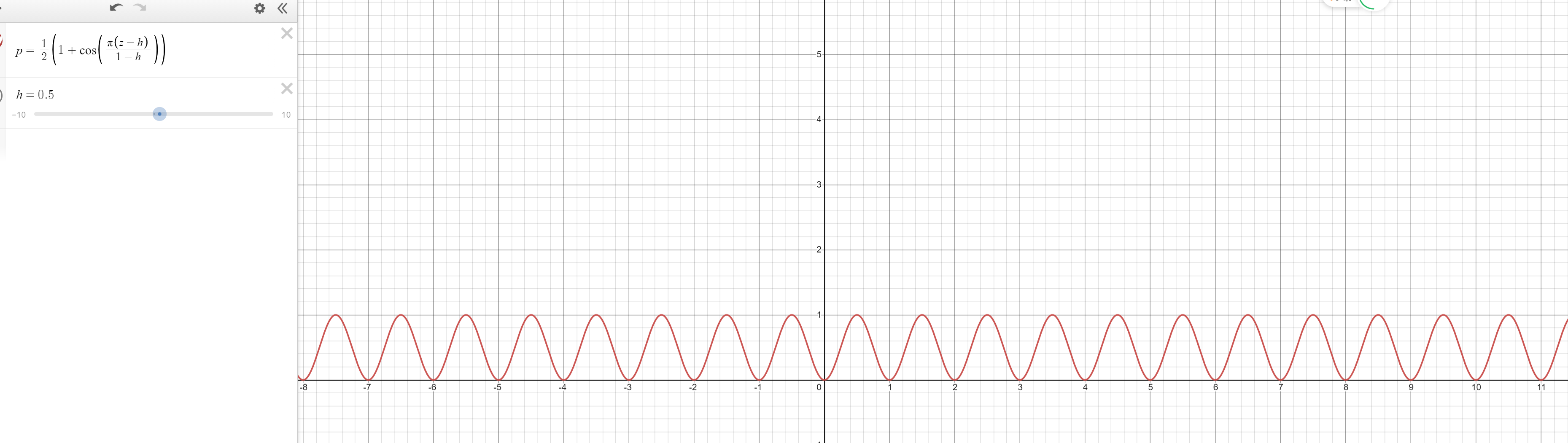
2. 使用bump function来建立smooth potential functions,避免折点且具有有限cut-off：

$$

$$

$$

$$

其中，\(h\in(0,1)\) ，在\(z\in[1,\infty)\) 时， \(|\rho^`_ {h}(z)|\) 是均匀分布在在Z上的。

也因为平滑的特性，继而定义平滑的空间邻接矩阵\(A(q)\)：

\[ a_ {i j}(q)=\rho_ {h}\left(\left\|q_ {j}-q_ {i}\right\|_ {\sigma} / r_ {\alpha}\right) \in[0,1], \quad j \neq i \]

其中\(r_{\alpha} = ||r_ {\sigma}||\)，对于所有的q和 i，\(a_ {ii}(q)=0\)

控制器模型：

\[ u_ {i}=f_ {i}^{g}+f_ {i}^{d}+f_ {i}^{\gamma} \]

\(f_{i}^{g}=-\nabla_ {q_ {i}} V(q)\)是微分项，代表对势能的微分，形成内部斥力

\(f^d_i\)是速度共识，代表形成共同的速度

\(f^{\gamma}_i\)是对群体目标的反馈

三种算法：

$(, ) $ 控制器

这种控制器只为形成\(\alpha -lattice\),即形成集群晶格，但是没有统一的目标和避障约束，所以容易分散，破碎成大小不同的若干个集群。

Algorithm 1: \(u_{i}=u_ {i}^{\alpha}\)

\[ u_ {i}^{\alpha}=\underbrace{\sum_ {j \in N_ {i}} \phi_ {\alpha}\left(\left\|q_ {j}-q_ {i}\right\|_ {\sigma}\right) \mathbf{n}_ {i j}}_ {\text {gradient-based term }}+\underbrace{\sum_ {j \in N_ {i}} a_ {i j}(q)\left(p_ {j}-p_ {i}\right)}_ {\text {consensus term }} \\ \mathbf{n}_ {i j}=\sigma_ {\epsilon}\left(q_ {j}-q_ {i}\right)=\left(q_ {j}-q_ {i} / \sqrt{1+\epsilon\left\|q_ {j}-q_ {i}\right\|^{2}}\right) \]

带群体目标的控制器

Algorithm 2: \(u_{i}=u_ {i}^{\alpha}+u_ {i}^{\gamma}\), or

\[ \begin{array}{r} u_ {i}=\sum_ {j \in N_ {i}} \phi_ {\alpha}\left(\left\|q_ {j}-q_ {i}\right\|_ {\sigma}\right) \mathbf{n}_ {i j}+\sum_ {j \in N_ {i}} a_ {i j}(q)\left(p_ {j}-p_ {i}\right) \\ +f_ {i}^{\gamma}\left(q_ {i}, p_ {i}, q_ {r}, p_ {r}\right) \end{array} \]

\[ \begin{aligned} u_ {i}^{\gamma} &:=f_ {i}^{\gamma}\left(q_ {i}, p_ {i}, q_ {r}, p_ {r}\right) \\ &=-c_ {1}\left(q_ {i}-q_ {r}\right)-c_ {2}\left(p_ {i}-p_ {r}\right) \end{aligned} \]

\[ \left(q_ {r}, p_ {r}\right) \in \mathbb{R}^{m} \times \mathbb{R}^{m} \text { is the state of a } \gamma \text {-agent. } \]

对于一个动态的\(\gamma-\text{agent}\)来说，可以有下列形式的控制器：

\[ \begin{array}{l} \dot{q}_ {r}=p_ {r} \\ \dot{p}_ {r}=f_ {r}\left(q_ {r}, p_ {r}\right) \end{array}. \]

如果\(\dot{p}_ {r}=0\)，则说明加速度为0，即集群将以一个固定的速度运动至固定目标点

带避障的控制器

\[ \begin{aligned} u_ {i}^{\alpha}=& c_ {1}^{\alpha} \sum_ {j \in N_ {i}^{\alpha}} \phi_ {\alpha}\left(\left\|q_ {j}-q_ {i}\right\|_ {\sigma}\right) \mathbf{n}_ {i, j} \\ &+c_ {2}^{\alpha} \sum_ {j \in N_ {i}^{\alpha}} a_ {i j}(q)\left(p_ {j}-p_ {i}\right) \\\\ u_ {i}^{\beta}=& c_ {1}^{\beta} \sum_ {k \in N_ {i}^{\beta}} \phi_ {\beta}\left(\left\|\hat{q}_ {i, k}-q_ {i}\right\|_ {\sigma}\right) \hat{\mathbf{n}}_ {i, k} \\ &+c_ {2}^{\beta} \sum_ {j \in N_ {i}^{\beta}} b_ {i, k}(q)\left(\hat{p}_ {i, k}-p_ {i}\right) \\\\ u_ {i}^{\gamma}=&-c_ {1}^{\gamma} \sigma_ {1}\left(q_ {i}-q_ {r}\right)-c_ {2}^{\gamma}\left(p_ {i}-p_ {r}\right) \end{aligned} \]

其中：

\[ \mathbf{n}_ {i j}=\frac{q_ {j}-q_ {i}}{\sqrt{1+\epsilon\left\|q_ {j}-q_ {i}\right\|^{2}}} \quad \hat{\mathbf{n}}_ {i, k}=\frac{\hat{q}_ {i, k}-q_ {i}}{\sqrt{1+\epsilon\left\|\hat{q}_ {i, k}-q_ {i}\right\|^{2}}} \]

这种控制器的难点是在于获取\(\gamma \text{-agent}\)的位置信息，对于圆型二维障碍物而言，可以有如下定论：

1. 对于一个拥有超平面边界且单位正交向量为 \(\mathbf{a}_{k}\)的障碍物， 并且该障碍物有点穿过位置 \(y_ {k}\), 则相对应的 \(\beta\)-agent 可以被确定为

\[ \hat{q}_ {i, k}=P q_ {i}+(I-P) y_ {k} \quad \hat{p}_ {i, k}=P p_ {i} \]

\(P=I-\mathbf{a}_{k} \mathbf{a}_ {k}^{T}\) 是映射矩阵（Projection matrix）

2. 对于以 \(R_{k}\)为半径，中心点在 \(y_ {k}\)的障碍物, \(\beta\)-agent的位置速度为：

\[ \hat{q}_ {i, k}=\mu q_ {i}+(1-\mu) y_ {k} \quad \hat{p}_ {i, k}=\mu P p_ {i} \]

where \(\mu=R_{k} /\left\|q_ {i}-y_{k}\right\|, \mathbf{a}_ {k}=\left(q_{i}-y_ {k}\right) /\left\|q_{i}-y_ {k}\right\|\), and \(P=I-\mathbf{a}_{k} \mathbf{a}_ {k}^{T}\)

代码使用的是定论2